
- within Finance and Banking topic(s)
- in United States
- with Finance and Tax Executives
- with readers working within the Advertising & Public Relations and Aerospace & Defence industries
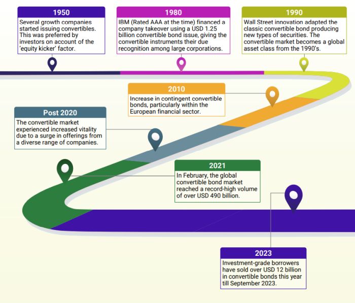
Convertible securities emerged during the nineteenth century in the U.S. This was during a period in which securing capital in a swiftly expanding nation posed several difficulties, which led to the incorporation of convertible clauses in mortgage bonds. This addition aimed to attract investors primarily for funding the railroad construction. Subsequently, several companies across various industries began adopting such financial instruments.
Owing to the increasing relevance of convertible debt instruments, it is crucial to understand the methods used to value convertible debt.
History of Convertible Debt Instruments
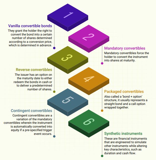
Types of Convertible Debt Instruments
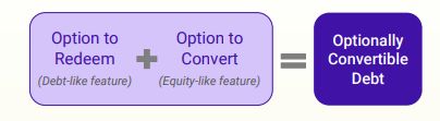
What are optionally convertible debt instruments?
In its simplest form, optionally convertible debt instruments are hybrid instruments that give the investor the option to:
- Hold the instrument to maturity and redeem it for par value or
- Exercise the conversion option and receive shares.
These are hybrid securities that have both debt-like and equity-like features. The arrangement can be equated to subscribing to the debt and buying a call option on the company's equity.
Complex convertible debt instruments can have features such as periodic call (redeemable) and/or put (retractable) features, or floating coupon rates, or are exchangeable into other exotic securities, or the underlying has an irregular dividend structure.
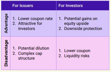
What are the advantages and disadvantages of optionally convertible debt instruments?
Valuation methods used to value optionally convertible debt instruments
The valuation of optionally convertible debt instruments varies from the valuation of a straight bond primarily due to the different pay-off structures based on the terms of the instrument.
The value of a convertible bond is the sum of two main components, namely, the value of the optionfree bond and the value of the options on the underlying instrument (generally common stock). The bond component is influenced by three main parameters, which are maturity, coupon rate, and yield to maturity (discount rate).
There are a variety of ways to model convertible instruments, including closed-form and numerical solutions.
- Closed-form solutions such as the Black Scholes Merton Model can only be used with a restricted set of assumptions. Therefore, numerical solutions are frequently used in practice.
- Numerical solutions such as lattice methods, finite difference methods, or Monte Carlo Simulations can include a path-dependent pay-off structure, allowing a more realistic implementation of convertible bond features.
In this article, we will discuss three widely used methods for valuing optionally convertible debt instruments:

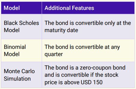
Black Scholes Merton Model
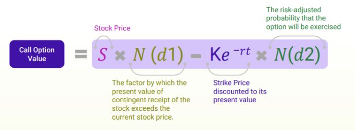
The Black Scholes Merton Model (BSM or Black Scholes) is a mathematical method used to calculate the theoretical value of an option contract, using six key inputs, namely current stock prices, expected dividends, the option's strike price, expected interest rates, time to expiration, and expected volatility.
The BSM Model assumes that instruments will have a log-normal distribution of prices following a random walk with constant drift and volatility.
The following equation is used to derive the price of a European-style call option:
Although the BSM Model can be used to value optionally convertible debt instruments with fixed maturity, for the valuation of complex debt instruments, the Black Scholes Model would not be an appropriate method. In this case, pathdependent models such as the Binomial Lattice Model or Monte Carlo Simulations are to be used.
Binomial Lattice Model
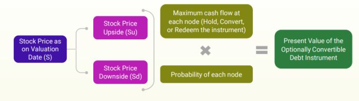
The Binomial Lattice Option Pricing Model is employed to calculate the value of an option using an iterative binomial framework. It is based on the presumption that the underlying asset's value follows a path of evolution. Hence, it either increases or decreases by a fixed percentage during each period.
Steps
- The first step is to build a binomial tree for the underlying asset
- Next, we construct an option tree where the intrinsic value of the option at each node is the maximum of the continuation value and the exercise value at each node
- Then we move backwards through the tree following a process known as backward induction to calculate the discounted value of the option at each node
- Finally, the iterative process continues by moving back one step at a time and repeating the procedure until the first node of the tree is reached. This will give us the value of the optionally convertible debt instrument as on the valuation date.
The Binomial Lattice Model is a powerful tool to build in complex features of the optionally convertible debt instrument. However, the model also has its own inherent weaknesses, including the fact that the binomial trees would require extensive computational capabilities for an option lattice based on non-recombining trees or to factor in multiple variables such as interest rate volatility, contingent conversion percentage, etc.
Monte Carlo Simulation
A Monte Carlo Simulation is a mathematical technique that simulates a range of possible outcomes for an uncertain event. These predictions are based on an estimated random range of values instead of a fixed set of values. This simulation becomes more accurate as the number of trials increases.
Steps
- The valuation of a convertible bond under the Monte Carlo
approach starts with simulating the underlying asset (which is
generally the common stock). The underlying asset is simulated
using an appropriate stochastic process, of which the most commonly
used ones are:
- Geometric Brownian Motion (GBM)
- Jump Diffusion Process
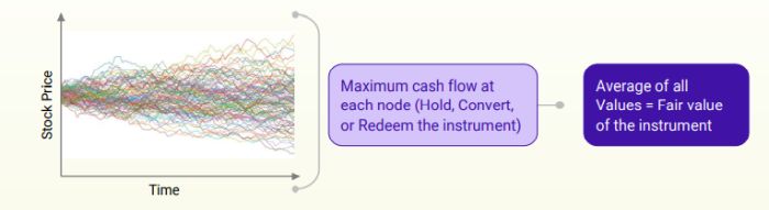
- The time to expiration is divided into equal time intervals and in each time interval, the stock price is simulated using an exact scheme. This procedure generates price paths and this process is repeated a certain number of times (known as trials).
- The maximum cash flow at each path is then determined and the average value of all trials will estimate the fair value of the optionally convertible debt instrument.
The Jump Diffusion Process is used to model an underlying asset that exhibits sudden shocks and jumps in value. It can be used to simulate stock prices of companies that experience sudden shocks, like those engaged in the oil and gas industry, or to factor in the chance of bankruptcy or disasters. In stock price modeling, due to the complexity involved in estimating parameters (especially for private companies), the GBM method is preferred.
Illustrations
For the purposes of this Illustration, we will consider an optionally convertible bond having the following features:
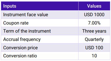
The market and stock-related information as on the valuation date were as follows:
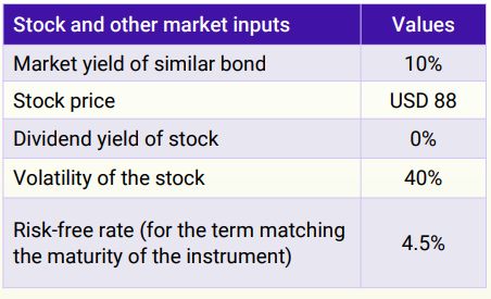
To present the capabilities of each model, we are using different terms for each model in addition to the features mentioned above.
We will estimate the value of this optionally convertible debt instrument using all three methodologies explained earlier with the above complexities.
Black Scholes Model
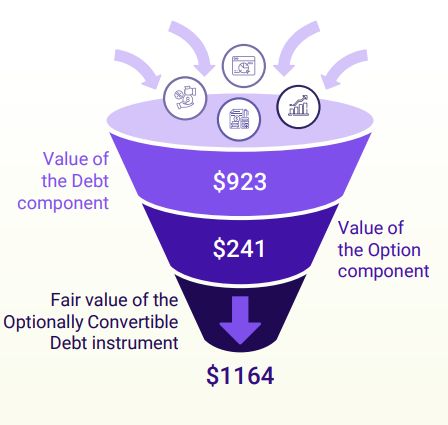
Under the Black Scholes Model, the value of the convertible bond is divided into two parts, namely:
- Value of the Debt component
- Value of the Option component
Note
- The value of the debt component is calculated by discounting the cash flows from the bond at the market yield of similar bonds.
- The value of the option component is arrived at by using the BSM equation, as discussed in an earlier section.
Binomial Lattice Model
A binomial tree of stock prices is constructed using the inputs for each quarter (period) as shown below:
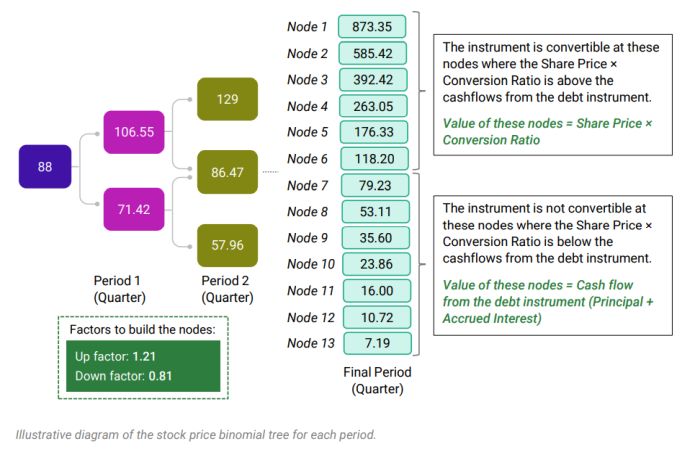
Using the methodology and steps mentioned earlier, we estimate that the fair value of the optionally convertible debt instrument is approximately USD 1,208.
Monte Carlo Simulations
The stock price at each period (quarter) is simulated through Monte Carlo Simulation using GBM. Examples of a few simulated stock price movements under Monte Carlo Simulations are shown below:
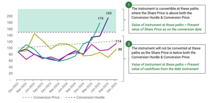
The value of the Debt Instrument is the average of all the cases (values determined under cases 1 and 2) We have used the methodology mentioned earlier and have run 1,00,000 stock simulations based on which we estimate that the fair value of the optionally convertible debt instrument is approximately $1225..
Valuation Requirements
Convertible debt instruments are subject to a range of regulations, accounting standards, and guidelines that establish a framework for financial reporting and disclosures.
US GAAP requires the fair value measurement of financial instruments. 'ASC 470-20: Debt with Conversion and Other Options' provides guidance on the accounting treatment of convertible debt instruments.
ASC 820 may require the issuer of the convertible note to bifurcate the fair value of the convertible bond into the fair value of the straight debt (liability portion) and the fair value of the conversion feature (equity portion).
The Securities and Exchange Commission (SEC) regulations also require companies to provide accurate and transparent financial information, including the fair value of their financial instruments.
The content of this article is intended to provide a general guide to the subject matter. Specialist advice should be sought about your specific circumstances.
