Breaking Down The Walls: A Series On Construction Delay Claims (Part 5 Of 6)

In the fast-paced world of construction, delays and disruptions can pose significant challenges to project success. In this Breaking Down the Walls series, Gary Brummer, a partner at Margie Strub Construction Law LLP, and Jacob Lokash, an associate at the firm, draw upon their extensive legal expertise to explore the complexities of construction delays. They have collaborated with Thomas Certo, Managing Director in the Construction Disputes and Advisory group at Ankura Consulting Group, LLC, whose insights into the technical aspects of delay analysis provide a comprehensive perspective on this critical issue.

Together, they simplify the fundamentals of construction delays, providing readers with the necessary tools to proactively identify and assess delays on their own projects in Canada. At the end of this six-part series, we will have explored the following topics:

1. Delay Claim Basics
2. Delay Damages
3. Disruption vs. Delay
4. Concurrent Delay
5. Forensic Schedule Analysis Techniques
6. Construction Delay Best Practices in Canada

Forensic Schedule Analysis Techniques

Thus far, this series has focused on providing readers with the requisite theoretical and legal framework to understand how delay claims are assembled and treated in an extension of time or prolongation cost claim. In Part 5, we turn our attention to the technical aspects of how delay is measured.

Quantifying delay requires a forensic analysis of past project events.¹ This article will outline how different industry publications² treat common Forensic Schedule Analysis (FSA) methodologies, including:

• As-Planned vs. As-Built
• Contemporaneous Period Analysis
• Retrospective Time Impact Analysis
• Collapsed As-Built Analysis

Defining Forensic Schedule Analysis

Before discussing the various methodologies, it is important to understand what FSA is, and what it aims to achieve. RP 29 offers the following introductory paragraphs on FSA:³

FSA is fundamentally a comparative exercise that seeks to understand how a project unfolded, and which events during the project execution may have impacted the project duration relative to the original planned execution. As highlighted in the above extract, there is some amount of subjectivity or "art" in FSA, which may lead to analysts having different conclusions on the same project.

The SCL Protocol similarly advises that an Extension of Time (EOT) assessment "should be based upon an appropriate delay analysis, the conclusions derived from which must be sound from a commonsense perspective." This "common sense" approach advises that an analysis should not be performed in a vacuum, and that the surrounding project circumstances must be considered when evaluating delay.

Some typical factors that lead to different FSA conclusions are:

• Review or availability of project documents beyond the project schedules
• Performance of supplementary supporting analyses (e.g., productivity analysis)⁴
• Application or interpretation of certain contractual provisions when guided by legal counsel
• Choice of an FSA methodology (and the application thereof)

Forensic Schedule Analysis Methodology Categories

RP 29 organizes the analysis methodologies into a hierarchical order.⁵ While the AACE taxonomy is quite detailed (and should be reviewed for a thorough understanding of all presented methodologies), the content is condensed in Figure 1, below.

All the methods discussed in RP 29 are retrospective in nature as they look back on the executed project or delay event(s). While prospective, or forward-looking, methodologies may be appropriate during an active project, they are not generally used when pursuing a delay claim after the fact.

The second level in the taxonomy distinguishes between Observational vs. Modeled methodologies:

• In an Observational technique, the analyst reviews the schedules "as-is". There is no effort to modify the project schedules in terms of activities, durations, or logic.⁶
• In a Modeled technique, the analyst actively modifies the project schedules to assess delay impacts. This may involve inserting or modifying activities, durations, or logic.

Lastly, each of the Observational and Modeled methodologies can be further categorized into specific methods.

• Observational methodologies utilize either Static or Dynamic logic:
  • Static logic analyses rely on the logic laid out in the baseline schedule without evaluating how that logic changed throughout the project schedule updates. This is described in RP 29 Method Implementation Protocols (MIPs) 3.1 and 3.2, and commonly referred to as an As-Planned vs. As-Built Analysis.
  • Dynamic logic analyses incorporate periodic schedule updates issued during the project. This allows the analyst to understand how logic and the critical path changed throughout the project. This is described in RP 29 MIPs 3.3, 3.4, and 3.5, and is commonly referred to as Contemporaneous Period Analysis.
    
• Modeled methodologies are either Additive or Subtractive:
  • Additive techniques insert delay activities, durations, and/or logic ties into the project schedules to observe if there is an impact on the project's finish date. This is described in RP 29 MIPs 3.6 and 3.7, and commonly referred to as a Retrospective Time Impact Analysis.
  • Subtractive techniques remove certain activities, durations, and/or logic ties from the project schedule to observe if there is a change to the project's finish date "but-for" given delay event(s). This is described in RP 29 MIPs 3.8 and 3.9 and commonly referred to as a Collapsed As-Built Analysis.

Practitioners should be cautious as terminology is often used interchangeably in the industry. For example, the term "As-Planned vs. As-Built Analysis" can be used to refer to any analysis that compares an as-planned schedule to its as-built counterpart and may not reference the specific methodology as described in RP 29. For this reason, RP 29 cautions against referring to methodologies by their common names and prefers reference in accordance with the taxonomy and MIPs.⁷ However, for purposes of this discussion and to keep the content simple, the authors will continue to use the common names.

Like RP 29, the SCL Protocol outlines various delay analysis methodologies.⁸ The SCL Protocol defines six "commonly used methods of delay analysis" including:

1. Impacted As-Planned Analysis
2. Time Impact Analysis
3. Time Slice Windows Analysis
4. As-Planned vs. As-Built Windows Analysis
5. Retrospective Longest Path Analysis
6. Collapsed As-Built Analysis⁹

The SCL Protocol contains summary-level descriptions of these methodologies and their implementation. While RP 29 tends to be more explicit about the nomenclature and implementation of various methodologies, there is overlap with the methodologies described in the SCL Protocol. Often, opposing experts relying on the two different publications can find common ground between their analyses.

The following sections outline how some of the more common methodologies attempt to answer the question of what was delayed and by how much. For any methodology, a root cause analysis may be performed to identify causation, or why a certain activity or scope of work was delayed. Finally, a review of the contract and entitlement, guided by legal counsel, will determine which party is ultimately responsible for a given delay.

As-Planned vs. As-Built

An As-Planned vs. As-Built (APAB) analysis compares the baseline project schedule (as-planned) to the schedule at the end of the project (as-built), and is performed in two general steps:

1. Identify the as-built critical path
2. Identify and quantify delay along the as-built critical path by comparing back to the as-planned schedule

Identifying the As-Built Critical Path

The determination of an as-built critical path is an integral part of the APAB methodology. Performing this step of the analysis allows identification of discrete delays to parties at the activity level of the schedule. Failure to identify the as-built critical path, and instead simply quantifying the overall delay, results in an APAB analysis that resembles a "Total Time" method, which is not a generally accepted methodology.

The as-built critical path represents what was driving completion during the execution of the project, or the longest path of activities from project start to project completion. There are several ways of identifying an as-built critical path, including:

• Retrospective Longest Path: Determine the as-built critical path by performing a backwards trace of work based on the as-built sequence of work
• As-Built Model: Build a forward-looking schedule network model incorporating the as-built schedule and determine the "forecast" critical path to be the as-built critical path
• Most Delayed Method: Compare the as-built dates to the baseline schedule late dates¹⁰ for any potential delayed work, possibly identifying multiple logic paths as critical in the as-built schedule
• Contemporaneous Causal Method: Identify the critical, driving activities on the data date of each contemporaneous schedule update. These activities, taken together over time, would represent the as-built critical path of the project.

Identify and Quantify Delay

Once the as-built critical path is determined, a comparison is made back to the baseline schedule for delay quantification. Figure 2 below illustrates a hypothetical as-planned and as-built schedule.

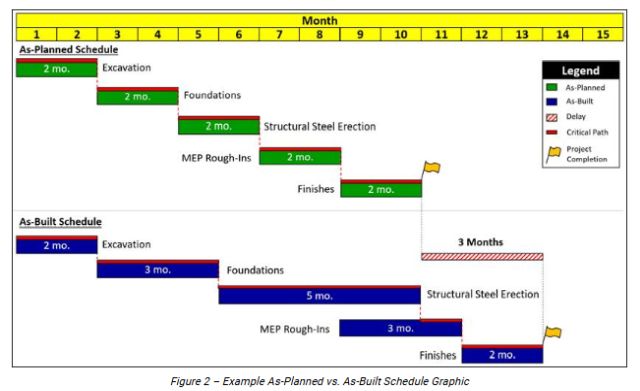
Figure 2 shows the as-planned construction sequence of excavation, foundations, structural steel erection, MEP rough-ins, and finishes, each with a two-month duration for a 10-month total duration. The as-built schedule shows that the project was completed in 13 months, for a total delay of three months. Using the APAB methodology, the three months of total delay can be separated into discrete impacts or mitigation efforts.

Stepping through the five construction activities, the delays encountered on the project were an extended duration of foundation construction (one-month delay) and the extended duration of structural steel erection (three-month delay). However, stacking of the MEP rough-ins to be partially executed while the structural steel erection was being completed eliminated a month delay (one month mitigation). Although the MEP rough-ins activity experienced an extended duration (one month longer than planned), the extended duration was mitigated by starting the MEP rough-ins early while the delayed structural steel erection was ongoing.

The analysis results are summarized and presented in Figure 3, below.

Figure 3 outlines how the various delays and mitigations to the discrete activities culminate in the three months of observed overall project delay. This parsing of the delay into discrete events allows the parties to understand the various contributors to the overall delay.

While the baseline schedule dates and sequence are typically agreed to between the parties, the as-built schedule information should be verified by contemporaneous documentation to improve analysis precision, when possible.

Contemporaneous Period Analysis

A Contemporaneous Period Analysis (CPA) considers the schedule updates that were developed periodically during the project to understand how the delay evolved over time according to the contemporaneous schedules. This contrasts with an APAB analysis, which only requires the baseline and final schedules (though more advanced implementations of the APAB consider the contemporaneous updates and incorporate the contemporaneous critical paths into their findings). The overall delay in a CPA will be the same as an APAB analysis, but the delay identification and quantification is instead developed through an update-by-update review of the schedules.

Over the course of a project, there may be numerous schedule updates, often at a prescribed frequency in accordance with the contract, typically monthly. The "period" in a Contemporaneous Period Analysis refers to the analyzed time between two schedule updates. The schedule updates will generally:

• Record as-built information for activities that started, progressed, and were completed to date
• Update the forecasted work through project completion

Therefore, a review of each period will include observations about how 1) as-built work progressed from the previous schedule update, and 2) changes to activities, durations, and logic of the forecasted works through project completion compared to the previous update. Incorporating a review of these logic changes over time differentiates the CPA as a "dynamic logic" approach compared to the "static logic" approach of an APAB analysis.

When implementing a CPA, RP 29 discusses three subtypes of the analysis:

1. As-Is (MIP 3.3): The analyst reviews the causes of a delayed or mitigated project completion date within a period by examining both the as-built progress and changes to the forecast schedule network. This exercise is completed between the Baseline and Schedule Update 1, between Schedule Update 1 and Schedule Update 2, and so on through to the end of the project.
2. Contemporaneous Split or Bifurcated Contemporaneous Period Analysis (BCPA) (MIP 3.4): This analysis focuses on as-built progress and sets aside forecast schedule network changes (non-progress revisions), as those events have not yet materialized. To implement this analysis between Schedule Update 1 and Schedule Update 2, the analyst updates the status of Schedule Update 1 (e.g., activity percent complete) with the status of Schedule Update 2. The result is a schedule with identical logic to Schedule Update 1, but stated with the as-built information and data date of Schedule Update 2. This process is referred to as a "half-step" and will show what the critical path and project completion date would be without non-progress revisions.
3. Modified or Recreated (MIP 3.5): This analysis aims to perform an "As-Is" or "Contemporaneous Split" method where contemporaneous schedule updates are not available. In this methodology, the analyst must use "updates that were extensively modified or 'updates' that were completely recreated."¹¹ After these schedule updates are created, an "As-Is" or "Contemporaneous Split" CPA can be executed.

The following sections outline how an analyst may implement an As-Is CPA and BCPA on an example project.

As-Is Contemporaneous Period Analysis

Figure 4 shows two monthly schedule updates ("Schedule Update A" and "Schedule Update B") on an example project:

Figure 4 depicts a period of an As-Is CPA analysis between two schedule updates:

• The top half of the graphic represents Schedule Update A that was issued at the end of Month 2
• The bottom half of the graphic represents Schedule Update B at the end of Month 3

A review of the as-built progress in Figure 4 reveals that the foundations, which were planned to be completed at the end of Month 3, were delayed by one month because of insufficient installation progress during the period. Moving beyond the Schedule Update B data date (represented by the green bars on the bottom half of the graphic), a review of the non-progress revisions shows that the revised plan for the Structural Steel Erection activity was extended by one month. Therefore, an As-Is CPA using these schedule updates would conclude that the project was delayed by two months during this period; one month of progress delay to foundations, and one month of non-progress revisions to structural steel erection.

While the As-Is CPA quantifies the delays from as-built progress and non-progress revisions separately, it does not observe the effect of the as-built (lack of) progress before non-progress revisions are made to the schedules.

Bifurcated Contemporaneous Period Analysis (BCPA)

A BCPA method takes the intermediate step to evaluate as-built progress prior to non-progress revisions. This is illustrated in Figure 5, below.

The top and bottom sections of Figure 5 show Schedule Updates A and B of an example project with no net delay during the analysis period. However, when a BCPA or "half-step" schedule is created by inserting the Schedule Update B progress into Schedule Update A (yellow-shaded portion of the graphic), an analyst can observe that there was one month of delay. The analysis conclusion for this period is that there was one month of as-built delay, which was offset by non-progress revisions. By making this intermediate update, an analyst can separately observe and quantify the effects of the non-progress revisions.

The BCPA is a powerful analysis tool that gives insight into the effects of non-progress revisions on schedule update completion dates. This additional analysis step gives the parties an understanding of what schedule revision decisions were made during the updates and can guide discussion on the feasibility of those decisions.

The CPA methodology utilizes what the parties reported during the project, which can be more appealing to a trier of fact than an APAB analysis, as this represents the best understanding of the parties at that point in time. However, care should be taken in evaluating the contemporaneous schedule updates. At times, non-progress revisions can be made that change the critical path and mitigate delay to project completion, even if those mitigation measures may not be achievable. Similarly, the schedule updates may fail to include delay impacts that are known to have occurred during the project, resulting in an analysis that does not account for the actual project events.

A review of the contemporaneous project record can assist the analyst in evaluating these schedules and adjusting the schedule where necessary to understand the project delays through a forensic analysis.

Retrospective Time Impact Analysis

We now move from the "Observational" techniques, which analyze project delay using unmodified schedules, to "Modeled" techniques, which add, remove, and/or adjust activities, logic, and/or durations to evaluate the impact of specific delay events.

A Time Impact Analysis (TIA) modifies the schedule by inserting an activity or series of activities (a fragnet) into the project schedules to understand the delay impact attributable to a specific event. A TIA can either be performed prospectively or retrospectively:

• Prospective TIA: When a potential delay event is identified, the delay fragnet is inserted into the schedule with an estimated resolution date. Any observed delay to project completion is associated with that event.
• Retrospective TIA: After the conclusion of a known delay event, the delay fragnet is inserted into the schedule (typically using the schedule update prior to the delay impact inception). The end date of the fragnet coincides with the actual end date of the event. Again, any observed delay to project completion is associated with that event.

Consider the example prospective TIA analysis illustrated in Figure 6, below:

The top half of Figure 6 is the as-planned critical path for the schedule update just prior to an impact event. The bottom half shows the critical path with a prospective impact event with a two-month estimated duration inserted into the schedule between the foundations and structural steel erection activities. The insertion of this two-month event results in two months of delay to project completion.

Implementing a TIA is a relatively straightforward methodology for analyzing the delay associated with a specific event. A Prospective TIA can be helpful for parties to understand the potential impact of an event when it arises. In fact, some contracts explicitly require the use of a Prospective TIA when a potential delay event is identified. This allows the parties to mutually work towards a resolution for the delay during the project.

Similar to the example above, a Retrospective TIA can be utilized to demonstrate the delay to the start of structural steel. Retrospective TIAs, however, are often criticized as an overly simplistic representation of project events, which ignores other events that may have contributed to critical path delay and does not analyze for concurrency. A retrospective TIA analysis is limited only to the events which are inserted into the schedule, and therefore any other developments during the project (e.g., delays to other, non-modeled works) cannot be observed in the analysis.

Collapsed As-Built Analysis

A Collapsed As-Built Analysis can be thought of as the inverse of a TIA. Instead of adding an activity or fragnet to an unimpacted schedule, the analyst removes the delay event from the as-built schedule. This is also referred to as a "but for" analysis: "'But for' the impact, the project would have finished earlier."

Consider the example project shown in Figure 7, below:

The top half of Figure 7 shows the as-built schedule of this example project, which experienced a two-month impact on the structural steel erection activity. Using the Collapsed As-Built methodology, the duration of this activity is reduced by two months. In turn, the analysis schedule shows that project completion would be completed two months earlier. Therefore, the analysis concludes that the impact event caused two months of delay to the project.

The Collapsed As-Built methodology faces criticism as a purely hypothetical version of what would have happened "but for" the removed delay. The analysis does not analyze whether the work would have progressed according to the hypothetical, or if that sequence of work was even feasible. Further, the Collapsed As-Built methodology may elevate a non-critical delay to critical by removing the actual critical events from the project timeline.

Selecting a Forensic Schedule Analysis Methodology

Given the multiple methodologies available to an analyst, how does one decide which methodology to implement? Although there is no single industry-agreed methodology, RP 29 lists 11 factors that may influence this decision, acknowledging the real-world scenarios in which these disputes arise:

1. Contractual Requirements
2. Purpose of Analysis
3. Source Data Availability and Reliability
4. Size of the Dispute
5. Complexity of the Dispute
6. Budget for Forensic Schedule Analysis
7. Time Allowed for Forensic Schedule Analysis
8. Expertise of the Forensic Analyst and Resources Available
9. Forum for Resolution and Audience
10. Legal or Procedural Requirements
11. Custom and Usage of Methods on the Project or the Case¹²

FSA is a dynamic field where developments can influence methodology selection. For example, some of the resource restrictions noted in the above factors can be overcome by embracing technological advancements such as software solutions and artificial intelligence tools. Similarly, court decisions can shift favor towards or away from certain methodologies.

Forensic Schedule Analysis Techniques in Canadian Courts

The Critical Path Method is a widely recognized and commonly used tool in construction projects to manage schedules, and courts in Canada have acknowledged its utility in analyzing delay claims. That said, Canadian courts have not prescribed that parties use one specific FSA methodology over the other.

In circumstances where the contract may not dictate the choice of methodology, courts have deferred to the opinions of forensic analysts on the most appropriate FSA methodology for any specific circumstances. Forensic analysts may disagree on the use of a specific FSA methodology, which may become an issue in dispute itself. Here, the courts may evaluate the experts' competing rationales for using one methodology over the other to determine which methodology is more suitable for the dispute.

Ultimately, the choice of methodology will depend on the specifics of the project, the available information, and the circumstances surrounding the delay.

Conclusion

Each FSA methodology offers its own advantages and limitations that should be carefully weighed when addressing delay claims. The industry guidance provides analysts with a toolkit designed to dissect project timelines and identify the causes of delay. A commonsense application of these methodologies can provide clarity in complex project disputes where time and cost overruns are in question.

As the FSA field continues to evolve, the integration of technological advancements such as specialized software and artificial intelligence presents opportunities to enhance the precision and efficiency of these analyses. This evolution not only aids in reducing subjectivity but also helps stakeholders manage resources in the face of growing complexity in modern projects.

Ultimately, FSA relies upon the analyst's ability to balance scientific rigor with professional judgment, considering contemporaneous records and the expert's experience. An experienced forensic schedule expert, coupled with knowledgeable legal counsel, will set stakeholders in the right direction to successfully evaluate delays on a project.

Footnotes

1. This process is typically retrospective and performed after the delay events have occurred. However, at times where a delay is forecasted or ongoing, a prospective, forward-looking, exercise may be necessary.

2. Namely, The Society of Construction Law ^{Delay and Disruption Protocol ("SCL Protocol"), and The Association for the Advancement of Cost Engineering International Recommended Practice No. 29R-03 Forensic Schedule Analysis ("RP 29").}

3. RP 29, Page 9.

4. At times, asymmetrical budget or time constraints between the parties may restrict an analyst's ability to perform detailed supplementary analyses.

5. RP 29, Page 12.

6. At times, minor adjustments to activities, logic, or durations are made in "Observational" analyses to account for documented inaccuracies (e.g., modifying an activity completion date supported by other contemporaneous documentation). A "Modeled" analysis refers to larger schedule adjustments to specifically isolate the analyzed delay.

7. RP 29, Page 11.

8. SCL Protocol, paragraph 11.4.

9. SCL Protocol, paragraphs 11.5 and 11.6.

10. An activity's "late dates" are the latest dates that an activity can start and finish without impacting project completion.

11. RP 29, Page 65.

12. RP 29, page 125.

The content of this article is intended to provide a general guide to the subject matter. Specialist advice should be sought about your specific circumstances.