Introduction
The IFRS 9 standard requires firms to quantify expectations of lifetime default risk and Expected Credit Losses (ECL) for certain financial instruments. The standard recognises that future losses are uncertain and asks firms to evaluate a range of possible outcomes to arrive at an estimate of expected loss that is "unbiased and probability-weighted" (paragraph 5.5.17).
Mathematically, the expectation of a random variable x can be computed using a continuous summation over all possible values of x and the probability p(x) of each value occurring, i.e. Ε[x] = ∫x p(x) dx.
Many banks have pursued an alternative approach, whereby the continuous range of possible scenarios is replaced with a finite number of forward-looking macroeconomic scenarios, and the loss severity estimated for each one. With enough macroeconomic scenarios, the expectation of the underlying distribution of credit losses can be materially recovered. This article explores approaches to recovering the expectation using numerical methods (assuming precise and certain input variables).
Definitions
We first define losses and their cumulative probabilities:
- Li represents the credit loss estimate (as a % of the book or in £ absolute terms) for a given scenario (this can be related to a state of the macroeconomy but can include idiosyncratic outcomes such as different recovery strategies by the bank).
- pi represents the cumulative probability of Li occurring (so the credit losses associate with a "1-in-7" upside scenario would have p=14%, or in other words 14% of credit loss outcomes will be more severe).
For a firm using three scenarios, the following data points are therefore available:
- (0,0) – zero probability of zero loss;
- (L1,p1) – some "upside" scenario;
- (L2,p2) – some "mid case" scenario;
- (L3,p3) – some "downside" or "stress" scenario; and
- (1,1) – the worst possible outcome is 100% (i.e. loss of the entire loan book).
These data points are in-effect samples on the cumulative distribution function (CDF) of losses F(L).
The expectation of a credit loss is defined as Ε[L] = ∫L f(L) dL where f(L) is the probability density function. Therefore, to determine the expectation, we must first determine f(L). By definition this is the derivative of the sampled CDF, i.e. f(L) = dF(L)/dL, and can be directly evaluated under various assumptions about the underlying functional form of f(∙). We explore in the following section, example assumptions:
1. Any symmetric distribution
In the event that the loss distribution is perfectly symmetric, then the median loss is equal to the mean (expected) loss as well as the mode (most likely) loss. If symmetry can be proven, then only a single, even-odds, scenario is required in order to recover the expectation of loss. In other words, if p2 = 0.5 then E[Loss] = L2 and no other information is required.
Although the zero-skew assumption might hold across a whole credit portfolio, it is unlikely to be true in granular cohorts or at all points in the economic cycle, which can lead to errors in granular reporting or disclosures. Nevertheless, over a third of respondents to our sixth annual IFRS banking survey stated that they planned to use only the most-likely scenario.
2. No Interpolation
Without evidence of a symmetric loss distribution, we may choose to weight the loss data points without attempting interpolation. This is equivalent to assuming that f(L) is non-zero at precisely three data points, and that the CDF resembles a staircase.

The expectation of the distribution can be recovered using the following formula:
In practice, the true loss distribution will never be non-zero at precisely three data points. The decision not to interpolate is therefore likely to fall short of "reasonable and supportable" per the IFRS 9 standard (paragraph 5.5.4).
3. Straight Line Interpolation
In this example, we present a linear interpolation approach. We draw straight lines between sampled points on the CDF, leading to a CDF that resembles a Trapezium:

The derivative of the CDF function can be calculated in each region of the CDF in order to determine f(L), the associated Probability Distribution Function (PDF).
With knowledge of f(L), the expectation of the loss distribution can then be recovered by evaluating ∫L f(L) dL using either Trapezium Rule integration, or the standard result that in a region of constant f(L) = k, bounded by (Lupper, LLower) then:

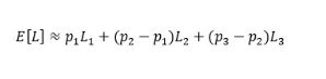
With the five data points described above, after gathering terms we obtain the following expression for the expectation:
This result is mathematically correct but the expression is dominated by the assumption that the worst possible loss is described by the data point (1,1). Banks would argue that IFRS 9 impairment should not double count capital requirements which in this instance (assuming 100% loss) would be the case. Another option would be to replace the final term(s) with data points obtained from an Economic Capital model. However, this can highlight potential inconsistencies and relies on sophisticated tail loss modelling capability.
Therefore, if the final term is removed, then the expected loss is materially recovered without the need for sophisticated tail loss modelling capability:

In many respects dropping the final term is an intuitive result: Many banks do not have Economic Capital (EC) models, but are still able to price for expected losses; and different EC models can and do give different results, without impacting the expectation.
Returning to the question of what is "reasonable and supportable", the presence of discontinuities in the CDF at each sample seems highly unlikely in practice, and again may fall short of what is "reasonable and supportable" per the IFRS 9 standard (paragraph 5.5.4).
4. Skew-Normal Interpolation
In this example, we present an approach without discontinuities in the assumed functional form. For illustration, we have assumed that the appropriate functional form is a skew-normal distribution. Note that the absolute optimal functional form may in theory be selected using Maximum Entropy. In practice, this would require considerably more data points and the assumption cannot be validated statistically.

The skew-normal distribution is described by three parameters:
- ξ – the location
- ω – the scale
- α – the shape
The parameters can be fitted using an optimisation approach to match our five sampled data points. The expectation recovered using the following closed-form solution:

Elegant though this function may be, its parameterisation would require a separate optimisation to be performed for every instrument (or homogeneous segment). Multiple optimisations may be operationally burdensome in a working day process. However, the approach can serve as a useful validation test to be performed offline in order to demonstrate that a bank's chosen interpolation approach does not lead to material bias.
Conclusions
We have presented four approaches for recovering the expectation a distribution from a finite number of loss data points. Indeed, it is likely that market participants will find alternative and equally plausible distributional assumption whose expectation is tractable.
It is nevertheless worth mentioning the orthogonal conclusion: Approaches which are not reconcilable to plausible distributional and interpolation assumptions cannot in general be relied upon to return accurate estimates of expected credit losses, at reporting dates across the economic cycle.
Finally, we revisit the assumption that the input variables are precise and certain. In practice, scenario features and the likelihood of each scenario's loss severity are not known with anything near complete certainty, and require experienced human judgement to calibrate. Significant variations between banks' impairment allowances under IFRS 9 therefore seem likely to emerge as banks publish their transitional impacts over the coming weeks.
The content of this article is intended to provide a general guide to the subject matter. Specialist advice should be sought about your specific circumstances.