Background
The IFRS 9 standard requires firms to quantify an unbiased expectation of credit losses (ECL) for in-scope instruments (IFRS9.5.5.17) that incorporates all reasonable and supportable information (IFRS9.5.5.4). As the transition date approaches, many firms have finalised their collective quantification approaches and, indeed, a consensus around modelling approaches may be beginning to appear.
For individually assessed exposures, however, there appears to be little consensus on what inputs to capture and how to process them in order to recover an unbiased expectation of credit losses. Nowhere is the risk of mis-statement more profound than in Commercial Real Estate (CRE), where future cash flows and capital value can be heavily influenced by idiosyncratic or heterogeneous factors.
In this article we focus on reducing error in CRE impairment estimates by modelling using granular indices which split the aggregate 'All Property Index' by location, sector and quality.
Introduction
Existing approaches to impairing defaulted Commercial Real Estate typically acquire an open market valuation as the basis for estimating losses. This valuation reflects the valuer's best estimate of the price that could be achieved in the market if the asset were to be sold on the valuation date. Empirical experience suggests that a same-day sale is a rare event. In practice, time is spent on renovations and marketing, as well as waiting for the sale process to complete. Uncertainty in timing and price lead to uncertainty in the present value of future cash flows.
Under IFRS 9, firms must explicitly consider a range of possible outcomes (IFRS9.5.5.17). To recover the expectation of uncertain future cash flows, it is tempting to apply an expected movement in the collateral index to all defaulted collateral valuations at reporting date. Indeed, under IAS 39, the most likely index movement is often applied. However, such an approach immediately presents two distinct sources of estimation error:
- Use of an expected or most likely index movement and time-to-sale represent a breach of the Jensen Inequality, which guarantees error in any use of an expectation "inside" a non-linear relationship. We discuss the Jensen Inequality in a previous article. This error can be overcome by estimating cash flows under a number of indexation scenarios (influencing indexed valuation) and recoveries strategies (influencing both time to sale, and indeed valuation).
- Use of a single aggregate index can mask significant divergence in asset values verses sector, location and asset quality specific indices. We explore the potential implications below.
Indexation Basis Risk
It is widely known, and accepted, that use of indices introduces basis risk into estimation. In retail (and retail-SME secured on residential property) lending, a large volume of largely homogeneous assets typically allows House Price Index (HPI) basis error to be modelled as unexplained variability or 'noise' in valuations. LGD Floor and Expected Shortfall models stand out as example approaches to quantification which avoid material bias.
By contrast, CRE assets are known to be considerably more heterogeneous than residential homes. For example, it is recognised by most firms that a CRE Index comprising, for example, prime office investments is unlikely to be suitable for secondary high-street shops or out-of-town shopping centres. The only comprehensive CRE indices available in the UK are MSCI indices, which comprise a relatively narrow pool of CRE assets held by institutional investment funds. Use of a single index to estimate forward sale prices for defaulted CRE exposures is therefore likely to bias estimation. Until now, the question of overall impact has not been explored in great depth.
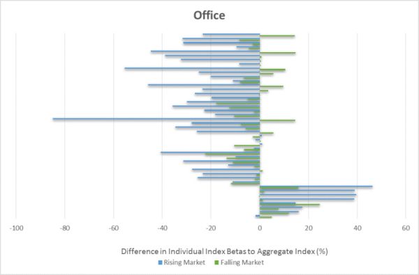
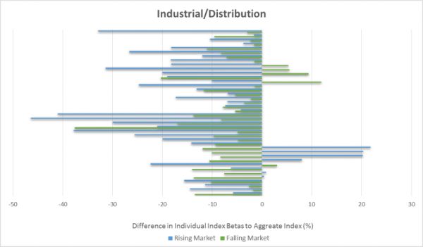
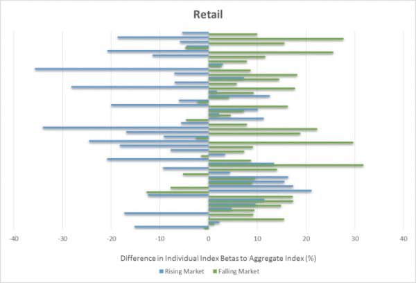
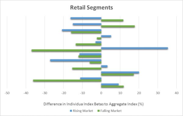
We analysed approximately 150 granular MSCI indices within the three main CRE sectors of Office, Industrial/Distribution and Retail using Panel Models with quarterly data from 2000 until 2017. We compared the first difference of the natural log of each index with that of the aggregate index or All Property Index (API). We found that the majority of the granular indices have experienced statistically significant divergence from the API which can largely be explained by three factors:
- Location – Some locations, on average, substantially outperformed the API whilst many have underperformed. Across all three main sectors analysed, there is a clear London/South East compared to Regional divide. For example, in rising markets, Central London offices outperform the API by approximately 40% whilst regional offices underperform by approximately 30%.
- Sub-sector – The retail sector is made up of diverse assets including shopping centres, retail warehouse parks, traditional 'high-street' shops and supermarkets. These sub-sectors demonstrate substantial variation in capital value movements. For example, supermarkets have been a relatively low volatility asset that declined in value on average 36% less than the API but increased in value 11% less. Contrast this to retail warehouse parks which have fallen in value on average 18% more than the API but have increased in value by 20% more. Another example is out-of-town compared to in-town shopping centres; in-town centres fell by 17% more than the API whereas out of town centres fell by 16% less, a 33% difference within one sub-sector.
- Quality – Across all sectors and locations there was a clear pattern of prime property falling less than secondary/tertiary property in a weak market and increasing in value faster in a rising market. In many cases, the difference was notable. For example, in a declining market, prime offices generally fall at similar rate to the API whereas weak secondary/tertiary offices fall approximately 15% more. A similar pattern is seen in rising markets, prime regional offices generally increase in value at a rate closer to the API whereas secondary/tertiary regional offices substantially under-perform. An extreme example is North West tertiary offices which, on average, increased in value 85% less than the API. Prime offices in this category increased only 25% less than the API which demonstrates a 60% difference within the same location/sector classification simply due to the quality of the asset.
The results are intuitive, and should not surprise anyone with experience of the CRE sector. When combined with knowledge that non-performing loans tend to be weighted towards secondary and/or regional assets, the results suggest that the accuracy of impairment estimates can be enhanced by moving away from single-index approaches to granular forward indexation.
The charts below display the results of the analysis in graphical form. The lines represent the percentage difference of the parameter estimate or 'beta' of a particular index compared to the aggregate 'All Property Index'. The blue lines show the difference when the overall market is rising and the green lines show the difference when the overall market is falling. A blue line in excess of zero means the individual index rises faster than the API and vice versa. A green line in excess of zero means the individual index falls faster than the API and vice versa.
The charts illustrate the extent of the divergence amongst indices which emphasises how an aggregate Index masks the performance of a diverse asset class.
Conclusion
We have shown that use of an All Property Index is likely to be inappropriate for any given CRE asset, and that higher-quality forward indexation can be achieved via use of granular indexation. Further, we would argue that this knowledge would constitute "reasonable and supportable information" per the IFRS 9 standard. In this context it is difficult to see how use of a single collateral index can be compliant. It is therefore incumbent on any lender using a single indexation approach to demonstrate that estimates have not been materially mis-stated as a result.
The content of this article is intended to provide a general guide to the subject matter. Specialist advice should be sought about your specific circumstances.